WK4DS Amateur Radio Blog
Search Posts
Smith Charts are easy…(The basics of antenna matching.)
When I decided to learn about Smith Charts and how to use them, I had no idea what a giant rabbit hole that was going to be. I have learned so much more since writing that first blog post about them that I wanted to revisit it and share some information with my readers. I love to learn new things and for some reason I have never taken the time (till recently that is…) to learn how to even read a smith chart, much less how to use them to design ANYTHING!
When I decided to learn about Smith Charts and how to use them, I had no idea what a giant rabbit hole that was going to be. I have learned so much more since writing that first blog post about them that I wanted to revisit it and share some information with my readers. I love to learn new things and for some reason I have never taken the time (till recently that is…) to learn how to even read a smith chart, much less how to use them to design ANYTHING!
The nanoVNA: A Vector Network Analyzer for everyone!
I started down this path with looking at antenna data from one of my POTA antennas on the nanoVNA. The nanoVNA is one of those wonders of modern technology that has become accessible to the masses recently. You see, before a few short years ago a VNA (Vector Network Analyzer) would easily run in the 5 figures and some of the nicer ones would break 6 figures. Rohde and Schwarz come to mind here… Even their used ones trade today for thousands of dollars…
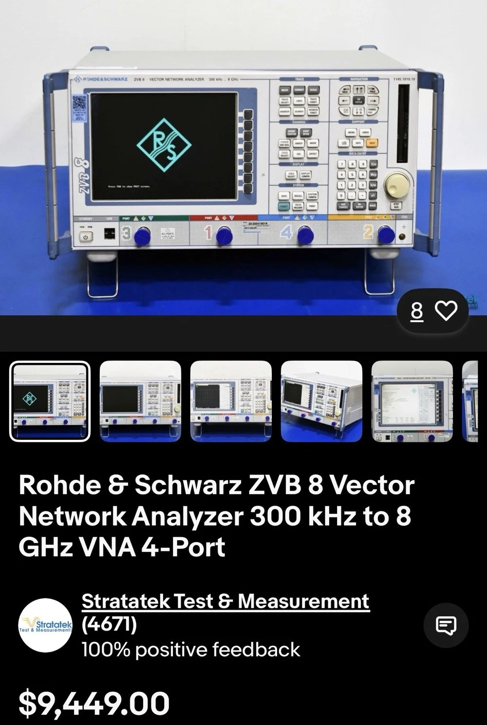
This is the reality of VNAs from just a couple of years ago. 4 and 5 figure prices for used units were common.
The nanoVNA changed all of that. It is small, runs on Linux and is now a single board computer in a tiny battery powered device that will literally sit in the palm of your hand. I have used one for my antenna setups for a couple of years now. I am actually on my second unit as the first one developed a fault and it was so inexpensive that I just bought a new one and threw the old one in the trash. You won’t see that happening with an HP / Agilent VNA!
There is a very good reason I use one for my antenna tuning needs too. The nanoVNA does everything those larger (and more expensive as well) ham radio specific antenna analyzers do that are available. You just have to learn a little more on how to use the nanoVNA. It also will perform functions that the antenna analyzers will not and this is where I love to bring the nanoVNA into the light. It has a smith chart function as well as an S21 input option that most, if not all ham radio antenna analyzers lack. You simply can not sweep filters with a MFJ antenna analyzer, at least not that I am aware of. This is where I found smith charts as I started to want to know what it was showing me on those charts. All of these nanoVNAs have a smith chart function and it is normally “on” when you start them up by default.
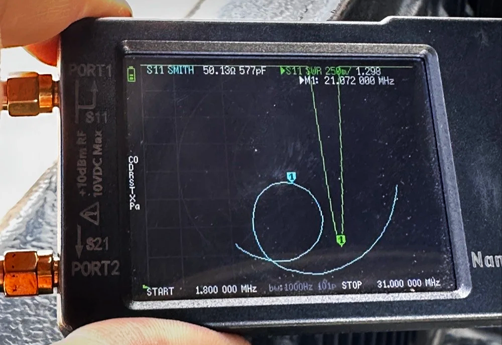
nanoVNA showing the Smith chart upon power up. Notice the diminutive size of the device compared to my fingers!
Smith Charts are NOT Scary…
In the above photo, the light blue trace is the one for the smith chart view. If you look really close, you can just barely make out the circular plot of the smith chart graph and in slight less illumination it does show up better. The light blue curved line represents the plotted values from 1.8 mhz up to 31 mhz (the two values are at the bottom) and you can move a marker along this plot as you go through that frequency range. In this photo I have stopped at 21.072 mhz as I was tuning my telescoping vertical to the 15 meter band to operate CW and FT8. It shows two more pieces of critical information though, the real reactance and the imaginary reactance..yes, imaginary… On these little nanoVNAs it shows up as either inductance (+j value when converted) and capacitance (-j value when converted). This antenna is measuring 50.13 ohms 577pf capacitive. We would need to convert this capacitance to a j value before we can plot it on the smith chart. I will get into that a little later in this article, but for now, this is a great tool if you are wanting to learn how smith charts work and I recommend you get one of these little wonders of technology for yourself and learn how to use it, even more so if you choose to use my link here to get it! As buying it from the link will help me maintain the website and costs you nothing extra.
One of my early attempts at working with a smith chart, it is covered in errors, but this is how you learn…
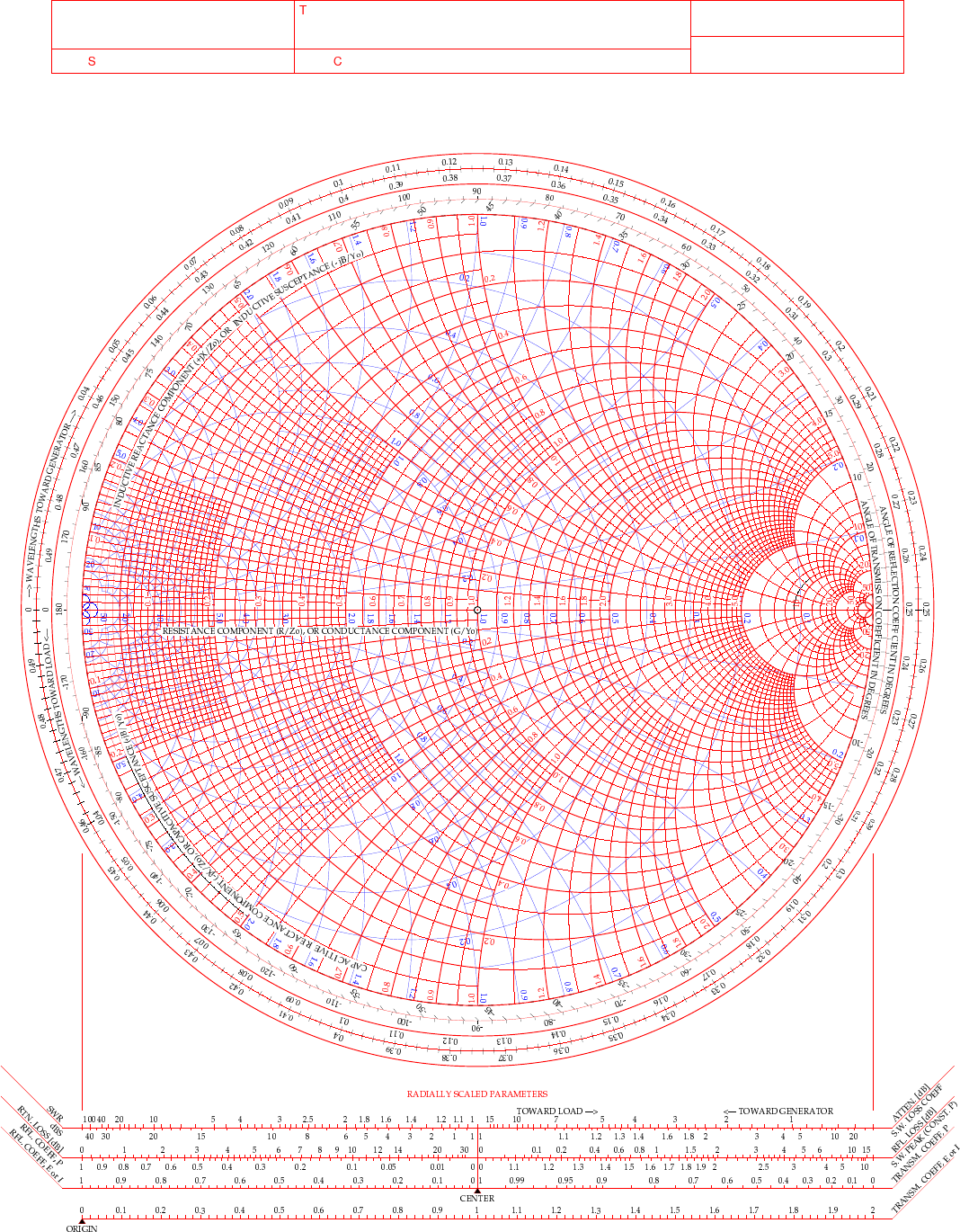
This is a plain, run of the mill smith chart (pictured above). This one shows two graphs in one chart. The red is the impedance graph and the blue one is the admittance graph.
Smith Chart: Understanding some basic concepts
The simple explanation for these two colors are as follows: red lines are series components and the blue are parallel components when you are using the chart for matching impedances between stages of devices. Like between the coax and the antenna as in the example I have drawn above. That is an antenna I use for POTA that I wanted to see what it would take to get it to 50 ohm resistive. (which is the point right in the middle of the chart BTW)
Already, I have given you three tidbits of intel about these charts and we haven’t even drawn on one yet… Another one is that the horizontal line through the middle is pure resistance and you will notice that it doesn’t say 50 ohms at the center, but rather the number 1. The chart is what is called “Normalized”. All this means is that you can assign what ever value you want to the chart and this center point becomes THAT number and all the others are relative to that value. Maybe you had two stages in an amplifier circuit that are 200 ohm impedance and you want to use this chart to match them, then the center is now 200 and you do simple math to get the other numbers from that point. Like the number 2 (moving to the right, remember we are using the red lines right now) will become 400 ohms as a result. Basically all the numbers are multipliers of the center value you assign. It really is that simple.
Fun fact: All the values below the resistive center line are capacitive and all the numbers above the line are inductive. So when you see one of those weird numbers like 117-j68 This is the “complex” impedance…duh, it even looks complex…haha. But to put it on the chart, it has to be what is called “normalized” and this simply means that you divide the first AND the second number by whatever you assigned to the center of the chart. For most ham radio and especially ham radio antenna stuff, this is 50 ohms. So this complex impedance normalized will be 117/50=2.34 AND 68/50=1.36. BUT since it is a negative “j” value it will now read 2.34-j1.36. This can be plotted on the smith chart directly now. The first number is ALWAYS found on the center “resistive” line first.Then after this point is found you find the second number on the perimeter ring as you see in the photo below. The reason I started at the bottom and not the top (which has the same exact numbers) is because it has a negative symbol in front of the letter “j”. If it is negative, it always goes in the bottom half and if it is positive, then it goes in the top half.
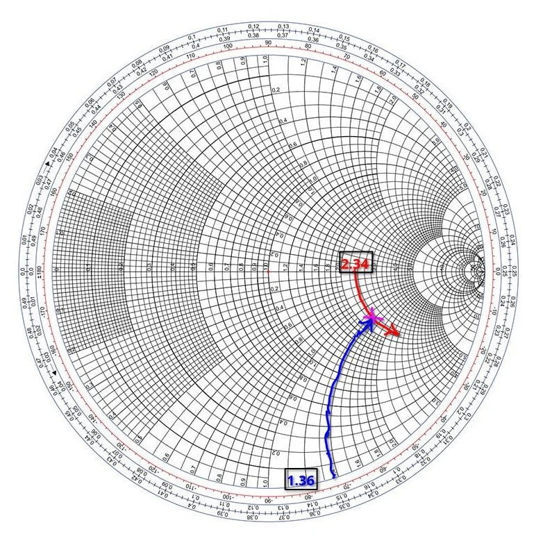
Smith chart showing the initial plot for the value 2.34-j1.36 and how to find it.
Then you simply follow the circular lines from each number out to where these two cross and this is your start point on the chart. Now this particular smith chart only shows the impedance curves so you need the second half (which is a literal mirror image of this one laid on top of it and in a different color) to be able to do a parallel → series type solution to solve for this. If we didn’t have the other half of the chart then we would never be able to put a component in parallel with the load as that is what the other half of the chart is for. Right now we can only add series components to get us up to the resistive line, but it will only give us the native resistance we started with and only eliminate the j portion of the value if we did that. It still doesn’t solve for the movement we need to get to 50 ohms resistive. I guess we could add a parallel resistor to lower the value, but that is really lossy option and we don’t want to put a resistor in parallel with our antenna, that is just burning RF and not putting it into the antenna. Remember a 50 ohm dummy load presents a perfect match to the transmitter output, but with radiate very little of that energy out to the world, instead it is turning this energy into heat…
Knowing this, the solution would be to add a “shunt” inductor to move the plot point up on the chart till it intersects the 50 ohm curve on the TOP HALF OF THE CHART. Once it intersects this line, we will add a series capacitor to bring the value back down to the center point, thereby matching the two stages perfectly. If this is clear as mud, then watch the video below for a visual explanation of what I just typed as well.
Add to all the stuff thus far the following tip as well, anytime you want to move the plot point up on the chart, towards the center line or above it, then you will use an inductor. By the same token, when you want to move the plot point down somewhere lower on the chart from where you are, you will use a capacitor. If you move along the red lines of the chart then it will be series with the load for either device (inductor or capacitor), if it follows a blue line then the device will be in parallel with the load. The below video by W2AEW does a really great job showing this visually so if you are a visual learner, this video is for you.
Matching Impedance with a Smith Chart…the easy way…
A good point someone made in one of the tutorials that I either read about or watched a video on said to remember you might need a specific solution for other reasons as well as to match impedance. Most of the time there is at least two ways to solve for these problems. In the example to follow below, I opted for a parallel capacitor and a series inductor, but let’s say you have two amplifier sections and you want to keep the DC voltage separated in the two stages, will then you would use a shunt inductor first then a series capacitor to finish the solution, this would match our impedance as well as block the DC voltage from the first stage as well. You see this is useful in more than one way.
Going back to the first image above of my hand drawn plot. If you will notice I drew a circle on that chart. This is called the Unity circle (for the reactance side) for some reason…. The point here is that no matter where you move the point along this circle the first number will always be 50. (If you used 50 ohms for that center point, from here on out I am going to assign 50 ohms to this value as that is what I use as a ham radio operator). Anywhere along this line, other than where it crosses the horizontal line in the center of the chart, there will be a “j” value added to it. If it is below the horizontal line, it will be negative and above will be positive “j” value. Now, at this point, if you want to use this chart to match a load, this is where the really easy stuff ends. Past this point you will need to use math…I know we have done some division earlier to get the normalized value so we could plot it above, but now we have to start calculating things like reactance and component values and such and as you know, this requires math… So buckle up as we match the 2.34-j1.36 mythical antenna from the second chart above to a 50 ohm transmitter output.
I have a two color chart below to make this happen as we have to use both colors to get it to work. The red dotted line is the arc on the impedance graph (red circles) for the 2.34 resistive value. You can see how I tracked it down into the negative region from the horizontal resistive line (this horizontal line is where you will always start these plots BTW) till it met the -1.36 blue dotted arc (denoted on the lower perimeter in red reactance arcs, you can see the numbers on the lower edge where I started). Yes, these charts are not precise to 5 decimal places, but are useful for ham radio ops and engineers use them for a myriad of other applications other than antenna matching like we are doing here. It will get you close enough to make the system usable and that is the whole point for us anyway. Anyway, these two initial lines meet at the start point of the process, the impedance of the antenna as measured…
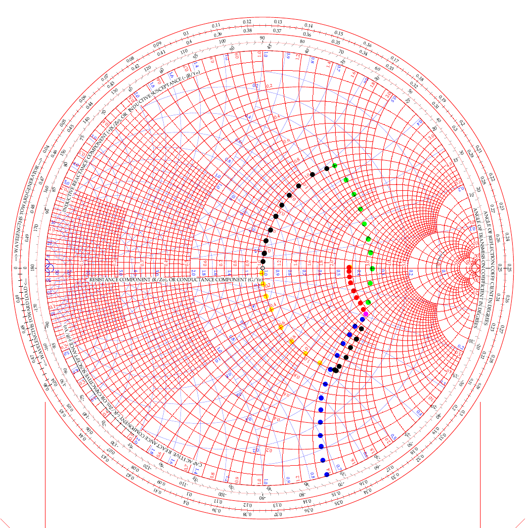
two color smith chart showing two possible ways to solve for L networks to match a transmitter to an antenna.
In the video above, he used the path of going up (like my green dots) and then following the 50 ohm arc back down (black dots from the green intersection point). But he was using a simple circuit built on a SMA connector. For an antenna installation though, it really makes more sense to me to actually follow the black line down from the start point and then follow the yellow line up the 50 ohm arc instead. Let me explain…
If we use the black arc that goes down first and the yellow one back to the center then what that looks like in the real world is a small capacitor from the base of the antenna to ground (this is what the black dotted line is after all). You see the black like is moving DOWN which means it will be a capacitor. We move it down till it meets the “50 ohm” circle so we can add the next part to move the point to the center of the chart. That next part isa series inductor between the base of the antenna and the coax. What us ham radio ops would call a load coil… This makes way more sense to me in this application than the other path which would be a “shunt” inductor or what would be an inductor from the antenna base to ground and then a series capacitor between the base and the coax. This is what would be similar to an L type antenna tuner to be honest but we are planning on using individual components in this lab… You see the yellow line is going UP to the central 50 ohm point, so this means it is an inductor and it is moving along the red lines on the chart which means it will be in series with the antenna.
This is actually really simple to be honest:
Red lines and your “movement” is going down - Series Capacitor
Red lines and your “movement” is going up - Series Inductor
Blue lines and your “movement” is going down - Shunt (Parallel) Capacitor
Blue lines and your “movement” is going up - Shunt (Parallel) Inductor
Do you see the pattern? Tracking up the lines on the chart is always inductors and tracking down on the lines is always capacitive. Like wise, if you use a blue line for your movement the the device will be in parallel and if the color of the line is red then it will be a series part. Now the color codes of my dotted lines above is purely there to make it easier to see what is happening and mean nothing other than that. The colors I am really concerned with are the two colors of the chart itself.
Math with a Smith Chart to match an Antenna
So the math is actually really simple to be honest. If you look at the first arc (the black line moving down) it is read on the blue chart (admittance - which is the opposite of resistance…) as it is moving along the blue circles. it is moving from about .19 to .48 on the blue chart (this is called suseptance, but you really don’t need to know that for this application) as you can see the lines run out to the perimeter where it is marked. This is .29 distance units on the admittance half of the chart. This .29 is the opposite of resistance so we then have to invert it (1 divided by .29), so it is a reactance value that we can use to do the math with, which turns it into 3.449 or as it should read -j3.449 (remember, because it is below the center line of the chart) and this is then multiplied by 50 (the value we assigned to the center point to start with) to get the actual reactance. 3.449 × 50 = 172.45 ohm of capacitive reactance. We now know everything in the formula to turn this into capacitance… since it is the same formula, you just switch out the two values. Super simple to be honest. Xc= 1/(2 x Pi x f x C) is turned into C=1/(2 x Pi x f x Xc) as you can see, we just plug in the numbers and then we get the capacitance. BTW, we are making this for 10 mhz so we can listen to WWV in Ft Collins… haha, why not?
Mathing this first step involved counting on the chart and subtracting the smaller number from the larger, then inverting it since it is on the blue lines (because the blue lines represent the opposite of resistance and we need it to be a resistance value), then multiplying that number by the center assigned value (in this example it is 50 ohms) and we ended up with 172.45 ohms of reactance. Now we turn this into C= 1/(2×3.1415×10e6×172.45) which is C=92.3pf
Once this step is done, we simply run up the red unity circle to the 50 ohm point in the middle and do the same thing but for inductance (since it is moving up on the chart). It looks like it is on about 1.42 on the red lines at the bottom of the chart, just take a look and see what I am talking about… Since it goes all the way up to the horizontal line, we just use this number and multiply it by the center value again (are you noticing a trend here yet?) and we get XL=1.42×50 so XL=71 ohms of reactance The we flip the inductive reactance formula and this time the formula looks a little different since it is XL=2 x Pi x f x L so to get inductance from inductive reactance the formula looks like this L=XL/(2 x Pi x f) so now we know all the numbers for this one too. It looks like this now L= 71/(2×3.1415×10e6) and this equals L=1.13uH of series inductance since this movement happened on the red lines and went UP.
So adding a 92.3pf shunt capacitor from the base of the antenna radiating element to ground (honestly an appropriately sized trimmer cap like a 50-100pf trimmer would be optimal since the calculated size is such an odd value...sure as a bird flies, this is some sort of common size…lol) Next is to insert a base “load” coil between the feedline and the antenna that is 1.13uH in size. This will match our mythical vertical to be resonant with the 10 mhz WWV signal as close to perfect as humans can get it. It SHOULD (if the parts are the right value) move the Smith chart plot to the center point on the chart which the goal for impedance matching.
Clear as mud again, right? HaHa… You can see it seems like a lot, but once you do it a couple of times, it really does get a lot easier to understand. I recommend you watch the video a couple of times and print off a chart from the web to practice on like this one.
Help support his website by using these Amazon Affiliate Links when you shop…
Smith Chart Exploration for Ham Radio: Building Impedance Matching Networks with DIY Inductors
Today finds the unsuspecting ham radio op perusing YouTube for something new to learn as it is really cold outside. He stumbles across a video about using a Smith Chart to match impedance and is intrigued…
What happens next is kinda terrifying…lol
Well to be honest, it is really kinda boring till you see how a smith chart sort of works and you start to learn how to use it to some degree. I have known about them for years, but have never understood how they work or even how to read them.
Today finds the unsuspecting ham radio op perusing YouTube for something new to learn as it is really cold outside. He stumbles across a video about using a Smith Chart to match impedance and is intrigued…
What happens next is kinda terrifying…lol
Well to be honest, it is really kinda boring till you see how a smith chart sort of works and you start to learn how to use it to some degree. I have known about them for years, but have never understood how they work or even how to read them. The other day though I landed on a video. This one shown below to be exact and I was hooked.
As you can see, if you watch this video, (maybe a couple of times), he explains it in simple enough terms that I actually understood what was going on finally! I did come into it with the understanding that the upper half was inductive and the lower half was capacitive from tuning my antennas with the nanoVNA. I would leave the smith chart on out of laziness and simply used the SWR graph to move the null to the operating frequency. But during this time, I started looking at the information presented on the display and noticed at times it would show capacitance and sometimes it would be inductance and also where the marker was sitting. This gave me the clue about what it was sharing with me. That was the extent of my smith chart knowledge though. At least it made sense to me. So the next logical thing to do was to order some smith chart notebooks from Amazon and a drawing compass so I could use said charts. While I was anxiously awaiting the new goodies to arrive, I started binge watching videos on smith chart use and taking away what I could from each video to add to what I already knew. By the time the paper arrived (I know I could have printed them off the web but the notebook format is really nice to be honest) {sarcasm}I was already a “master” at these “simple” charts… haha. {/sarcasm}
I will be honest with you. There is so much about these charts that I still don’t understand that it boggles the mind, but I have figured out how to use them for impedance matching and it is kinda awesome. I actually made the last few pages in my new notebook a cheat sheet based on the above video so I could reference it easily without having to watch the video over and over. I am absolutely going to build one of these fixtures when I get back home too. I would already have done it but I am not able to access my bench to put it together… So what follows is what you do when you don’t have that gear handy.
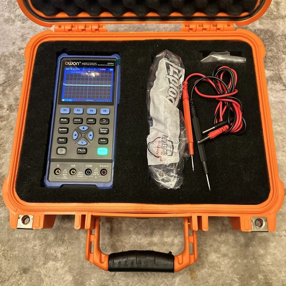
First things first, I bought a new toy. This is a 200 mhz “scope meter” but this one has another trick it can exploit. This is a actual dual channel oscilloscope AND it also has a arbitrary waveform generator as well! On top of the usual multi-meter functions as well. This thing has a lot to offer…till it doesn’t. It didn’t take long to figure out that the waveform generator doesn’t have the sweep function in it, this would have been nice to play with things. I can’t find FFT modes anywhere in it either so it can’t be a “poor man’s spectrum analyzer”. The little meter does have enough options to be really useful for what I was doing anyway so let’s get started… oh, it doesn’t come in this nice hardshell case. This is an Apache case from Harbor Freight. It is the perfect storage container in my opinion and I am happy to have it trimmed out like this. It didn’t take too long to figure out how to use the oscilloscope and I made a cheat sheet for it too so I can access useful features more easily in the future since a lot of it is hidden in menus due to the diminutive size.
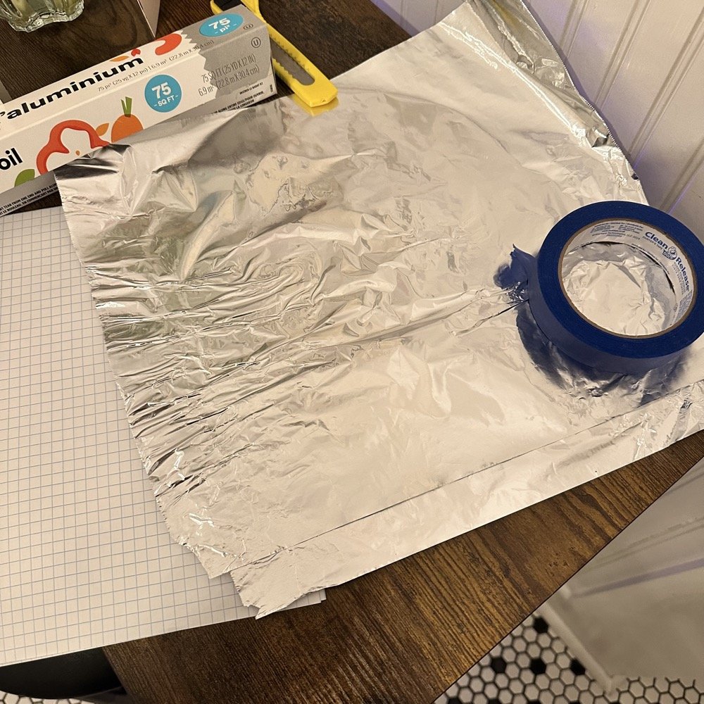
What you see here is pure desperation to see if I can make this smith chart stuff work for me. I am literally about to start making capacitors out of aluminum foil, a sheet of notebook paper and painters tape… Spoiler alert, it worked… You see, in another video I found on YouTube, there was this idea that you don’t need a LCR meter to measure your components as long as you have a known value device, a battery and some ingenuity. I also had a lot of time to play with this concept so here we are… I started by making a really big capacitor to start with to do a proof of concept and to see if there was enough capacitance to make this project work. Turns out there was way more than needed with the initial design, WAY more. So with the proof of concept made from three full size sheets of paper laminated with aluminum foil on one side of each one and then stacked so that the center sheet was one plate and the top and bottom were the opposite plate, I found I had made a .0034uF capacitor! This was more than enough to play with HF radio RF frequencies!!! Woohoo! Now this is all based on me being able to believe my new meter and later I find out that there is 17pf of stray capacitance in my meter and leads. Once I figure this out, and factor it into my math, it is all good but for now with this thing being 3408pf, I don’t think it is really a problem. The cigar box is there to use gravity to apply an even pressure to the “plates” and hold them at a consistent spacing as at this point, these were just three sheets stacked up. The top and bottom are connected to the black lead and the middle one is connected to the red lead. Also tested it with just on plate on the black lead and yep… capacitance went WAY down, so this style of capacitor worked pretty well to be honest. I could make it go up a good bit more by pressing on the cigar box too, I saw 5.0nF at one point while playing with it, that is crazy to me…
I had read somewhere about this idea to be honest. Well a cruder version of it actually. They made an impromptu antenna L network with two sheets of aluminum foil and a sheet of news paper or something like that. That made the capacitor and the inductor was wound on something found commonly in the house in the 1960s or 70s as well. They just used regular old romex house wire to make the inductor and it also worked just fine. Sometimes you just really need to have some “want to” and it can be done. I was a little more superfluous with my build as I didn’t need it to get on the air but rather as an experiment to see what I could learn.I honestly was really surprised to see how much capacitance I could get out of notebook paper and aluminum foil from the grocery store. This tells me that literally anyone that needs an antenna tuner, has one if they want it bad enough. You don’t have to have a Ten Tec 238 to be able to tune that random wire, you just need to gather some stuff you probably already have in the house…
Side note, I also finally acquired a new case for my POTA Scout 555 radio. I still need to finish the pockets for the band modules when I get home, but I now have it in a proper case and not just sitting in a cardboard box in the back of the truck! Also, I made another 60 meter contact today… to the same exact person that I made the first one with a couple weeks back! HAHA! I think we are the only two people on 60 meters CW in the mornings ever…
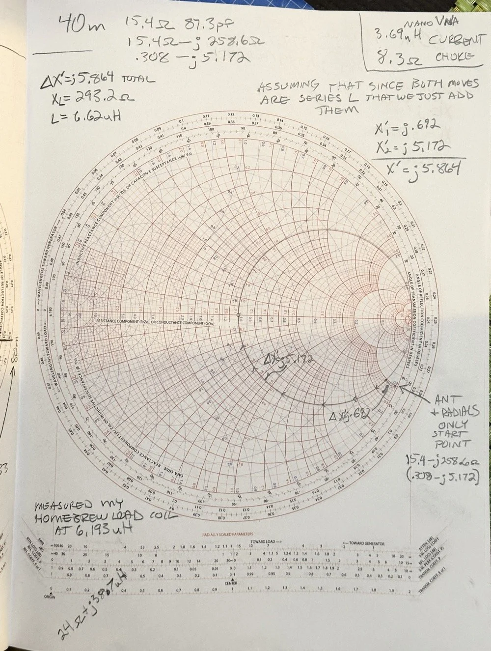
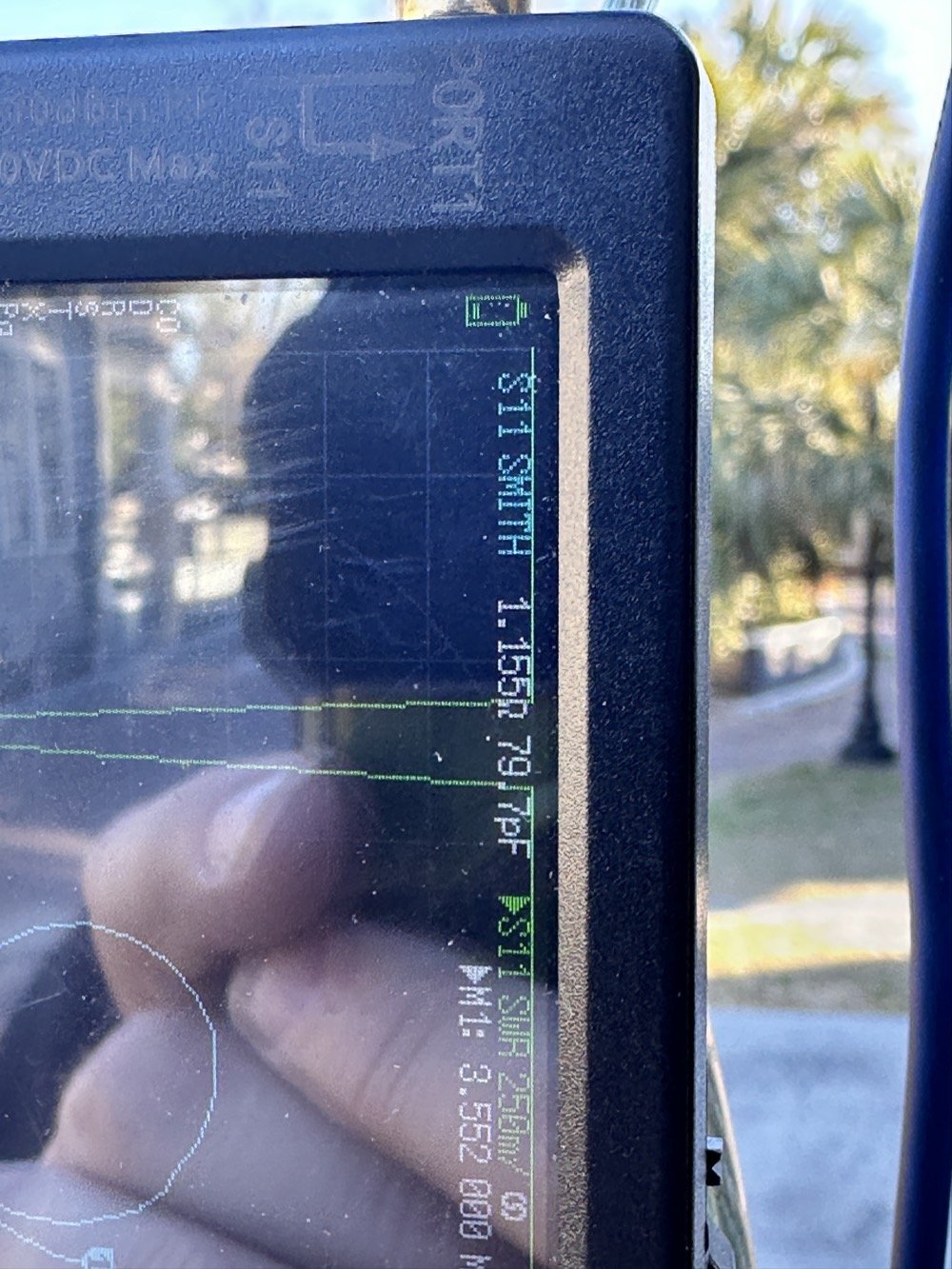
Here we see what I measured the other day while at a POTA park. What these numbers show is the antenna measurements for the band at the base of the antenna. I literally took the nanoVNA and adapted it to the antenna socket directly to eliminate the 50 ohm feedline from interacting with the measurement. As we will learn soon enough that you can use a piece of feedline (coax in particular) to move the base value around the smith chart should you need the starting point to be somewhere else. But I also learned something else about these starting point numbers below that I will share with you in a little bit.
At the top of the page, right next to the “40m” is what the nanoVNA reported that day at the park. (15.4 ohms and 87.3pf) you have to have two coordinates to plot anything on a chart so these are the two numbers you need to plot your starting point. Ignore the other notes as I am probably wrong on some of it and it actually makes more sense later. But the first thing I had to do was to turn these numbers into the proper numbers that the smith chart uses. This is called normalizing them. You see the chart is relative, you can assign whatever value you want to the center point on the chart and the rest of the chart is “relative” to this value. So if you were to work with 75 ohm coax and wanted to make an impedance matching network to work with it and having minimal losses, then you would assign 75 ohms to the center point. Since we use 50 ohms in almost all amateur radio (if not all) then our value is 50 ohms at the center point.
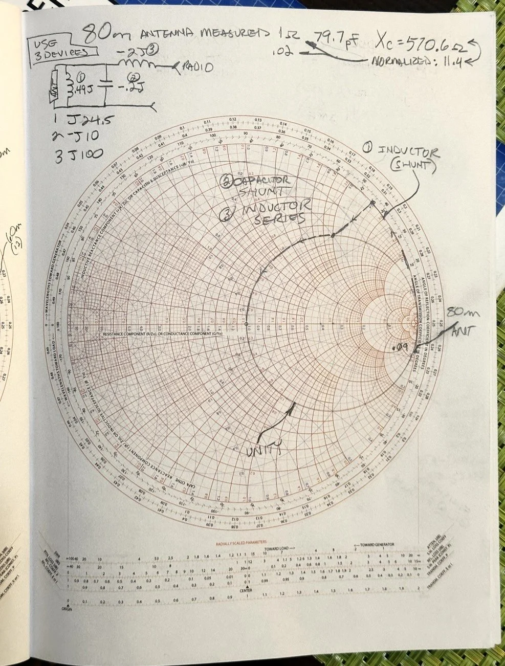
So here is my 80 meter plot (below) to get to a 50 ohm impedance from where it started at… yes… 1 ohm and 79.7pf capacitive! You see I am designing a matching network to couple my 50 ohm coax to a 18.4 feet tall telescoping vertical with a couple of radials thrown out on the ground. This is not even close to a matching antenna for the 80 meter band at all. Hence the terrible numbers to start with. Well, this was like those jokes you here from high school where you get something simple in the lecture in class about a subject then in the book it might show it with one more complication but the exam shows the Drake equation for the problem on the test! Well this is what happened to me as in the video above, the number in the video was closer to the middle of the lower half of the chart making for a more straight forward solution to the problem. I also did my admittance math wrong too if I am right…lol… since it is all inverted, but this doesn’t matter at this time. What you need to know at this point is that my problem lies outside the unity circle (that is the one I drew on the chart) and I need my “arc of movement” to cross this circle… it does but nearly at the infinity point (on the right side of the chart) which makes the math almost worthless… The reason the math gets pretty inaccurate is the numbers on the chart start getting logarithmic is value and so a small movement on the chart in this area makes huge changes in the values. You want your plot point anywhere else but here, yet this is where I am at in this blog post… haha
Knowing all this, I start this complicated, 3 position move to get me to the center of the chart. Mind you, I think this would actually work, but I am not sure if the math is mathing right at this time. (I am thinking the first move is a piece of transmission line to move the start point around the circle instead of an inductor and the second movement is also not a capacitor either so basically this whole thing is drawn wrong…lol) You will see why in a minute too as to why I dont know. The schematic for this movement is scrawled in the upper left hand corner of the notebook page if you wondered what it would look like to make this circuit. Two inductors and a capacitor to get to 50 ohms… how many antenna tuners have TWO inductors in them? I will help you out here… not many, if any. The number of inductors alone would make this a no go design for the most part unless is was going to be a one band wonder. Just remember I am pretty sure the math on this is wrong, the plot directions are correct, but I am thinking that the suseptance values are needing to be inverted to calculate the impedance for the two movements on the blue lines. Anyway, the point of this blog post is to show what is possible if you want to learn something new and it is not about the math around a smith chart…yet…lol I am diving back into the tutorials to figure out the blue part of the chart next.
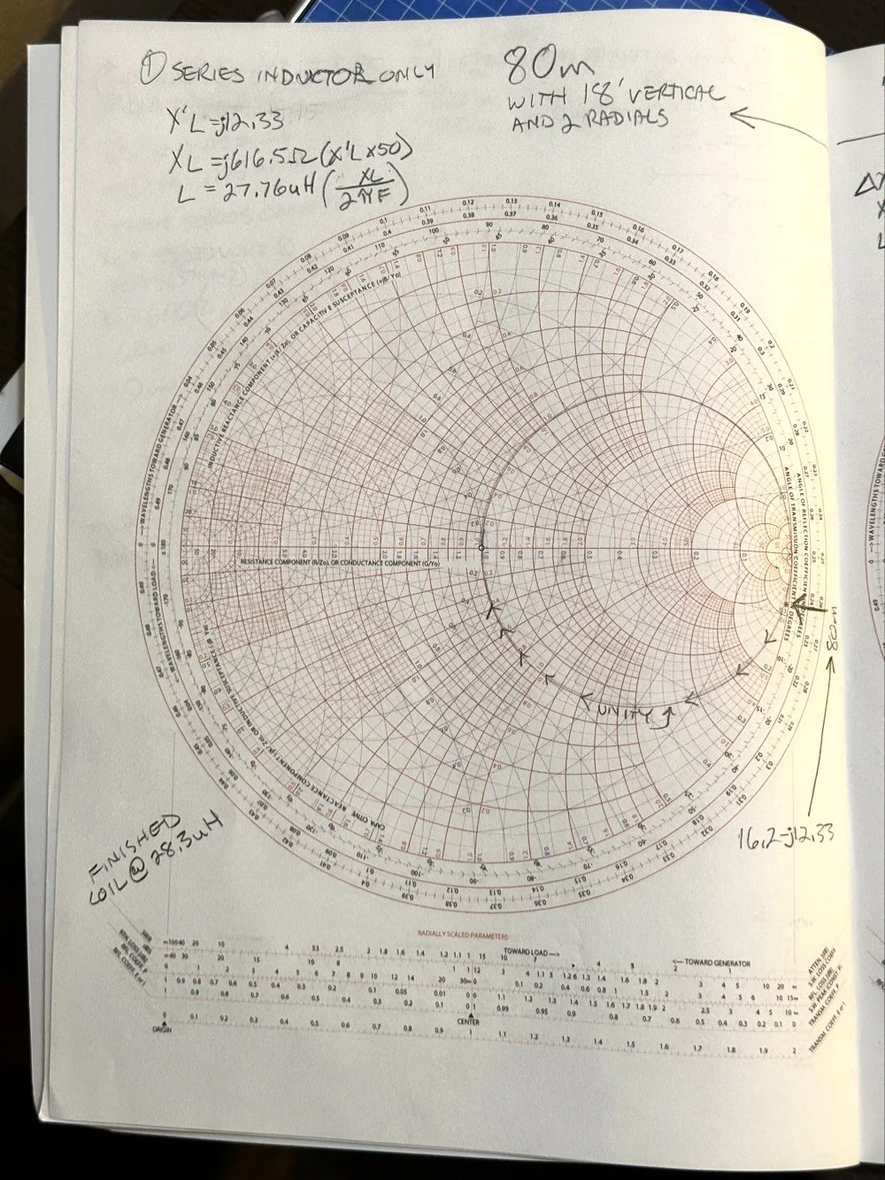
After I pulled my hair out for a while…wait, that don’t apply to me…I’m bald already… After getting over the frustration of trying to solve this problem, I redrew it on a fresh page and looked hard at it for a minute and had an epiphany… The plot point is not INSIDE the circle, or even anywhere closer to the middle of the chart at all, which would have been ideal, BUT it is really close to the unity line already. I mean REALLY close, so close in fact, I bet you could simply run around the unity line clockwise to the center point and just “eat” the misalignment on the horizontal resistance line of such a tiny amount and no one would even notice in the real world. You know what this matching network now looks like? A huge by large inductor is what, just a plain ole gigantic coil… Moving clockwise around the impedance lines (the red ones) indicates adding inductance to solve the problem. This is what all the antenna companies use when you buy a mobile 80 meter whip antenna if you think about it, just a huge load coil and nothing more. If you were to zoom in on this, I am guessing the resistive value when you get to the end of the arc, at the horizontal center line (which is the pure resistance line) would be something like 49.2 ohms or something close to that, literally less than 1.1 : 1 SWR maybe less to be honest.
Armed with this knowledge, I wanted to test this theory. So I now needed a way to make a coil to insert between the feedline and the base of the vertical to see if I had learned anything. Well I had this new scope / meter / signal generator widget and I had a way to make a capacitor, I then remembered a video where I guy showed how to measure inductors and capacitors with only a oscilloscope if you have one known device. Well, I have a capacitor that I made and I can measure it with the new meter, so that will give me the “known”.
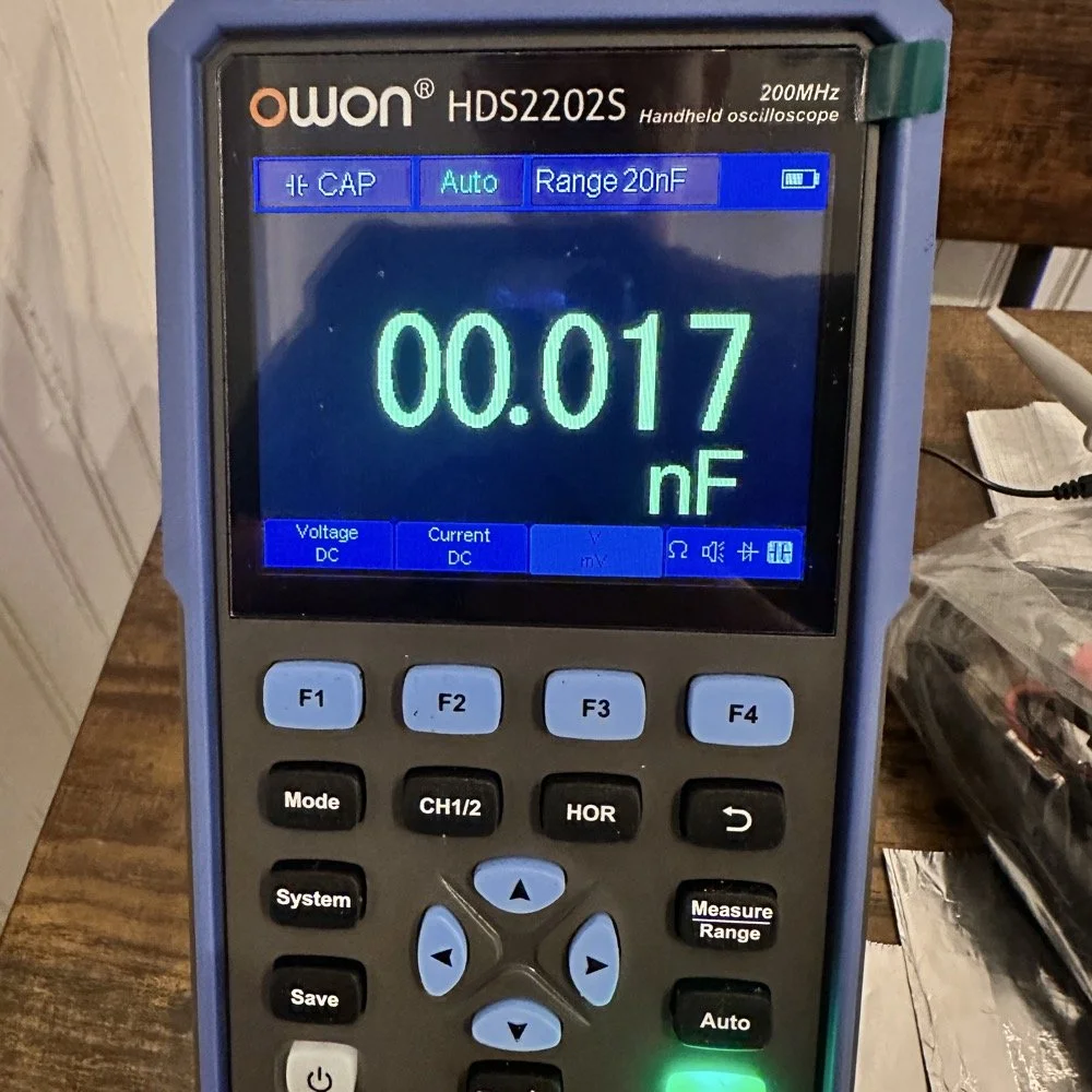
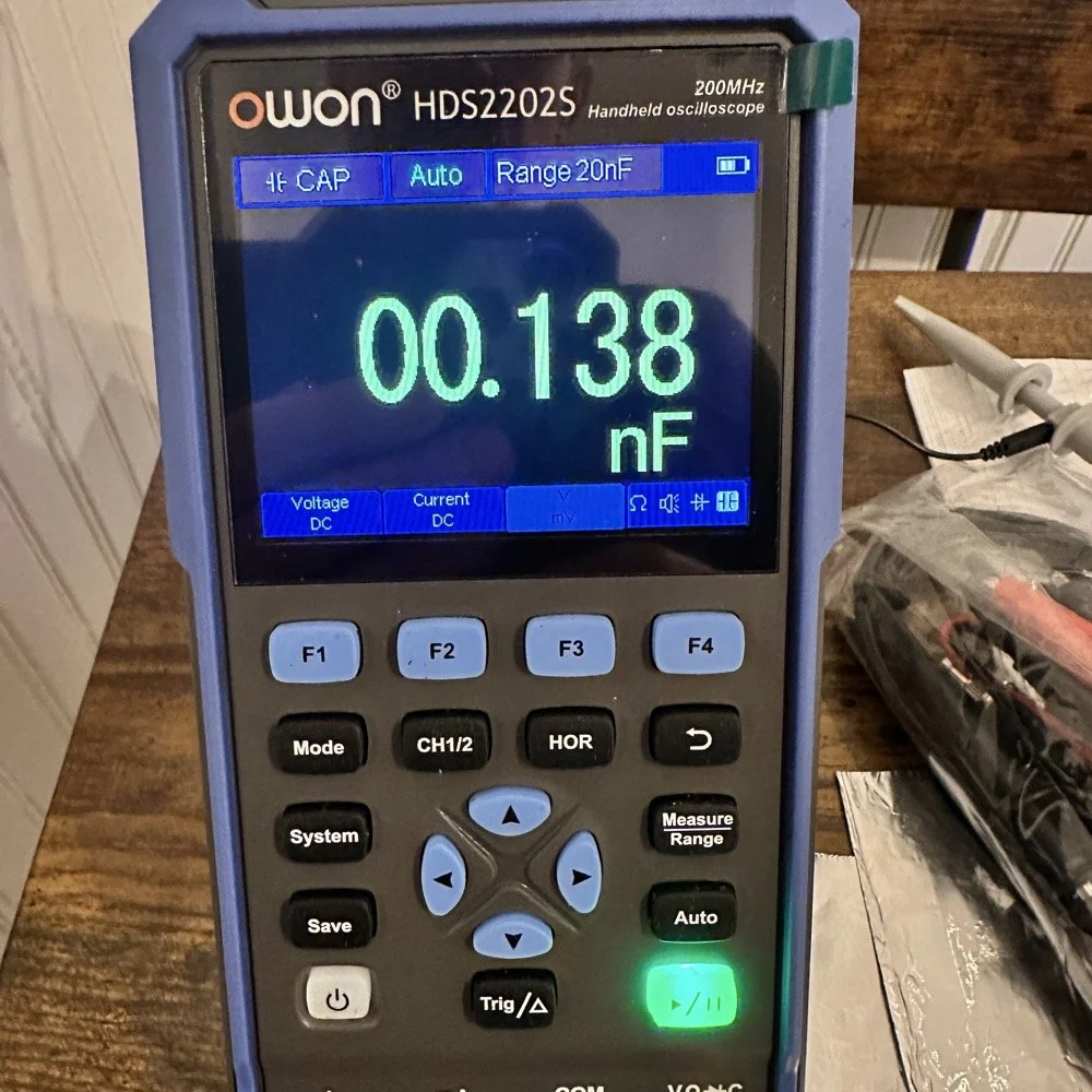
So I fire up the new meter and plug in the leads and find this. There is no way to “tare” out this number either so you simply have to subtract it from what ever you measure. I figured this would be pretty easy so I just went with it. Below is a photo while I was trimming the capacitor to a size I wanted. I was looking for 100pf and as you can see below on the meter, I was getting close. This is measuring right at 121pf in the photo. I would trim off the edge of the sheet and then check it again, rinse and repeat till it was close to what I wanted.
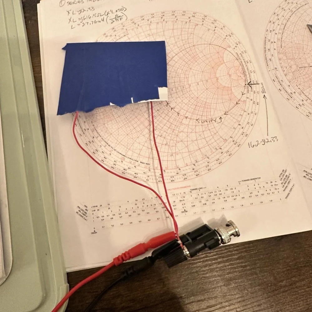
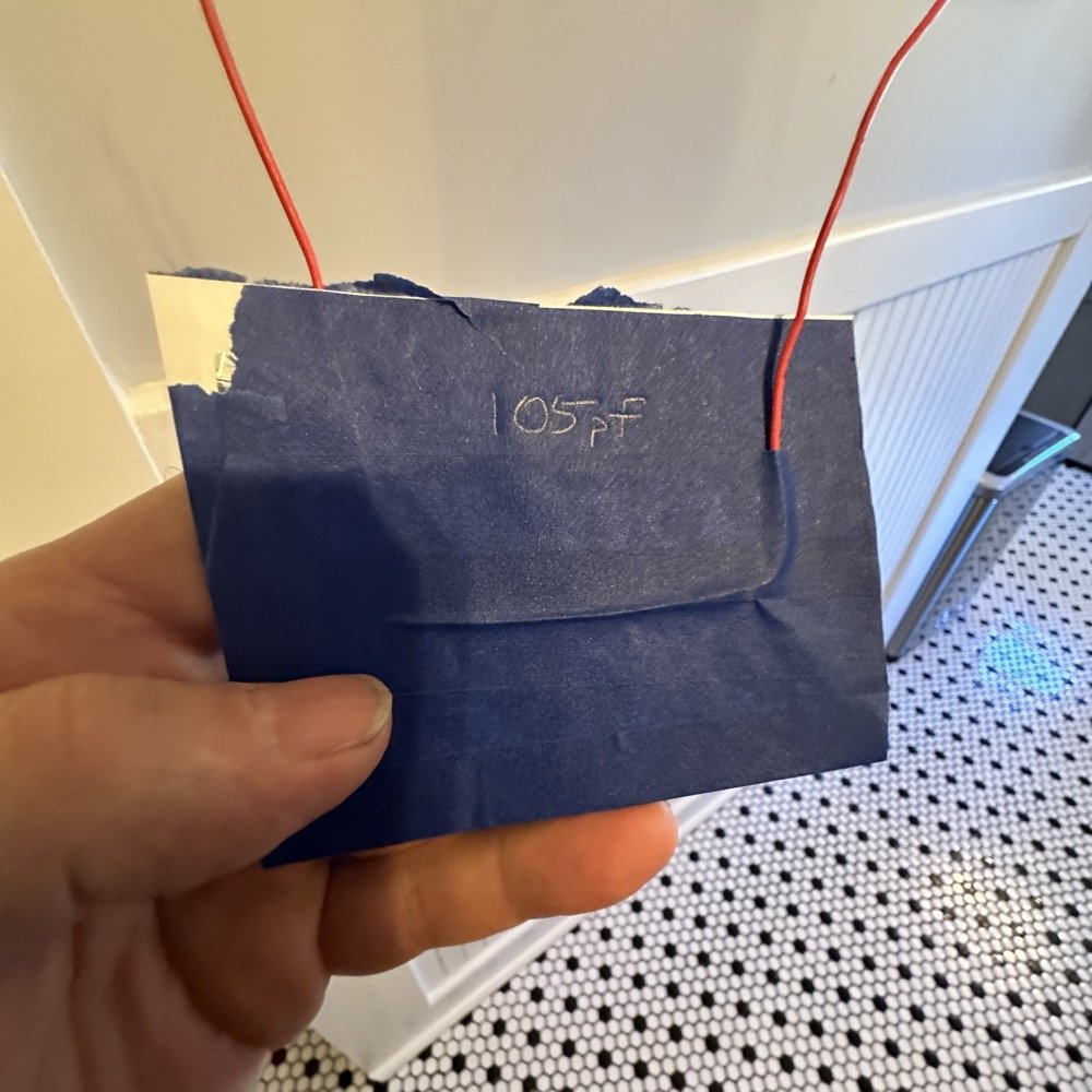
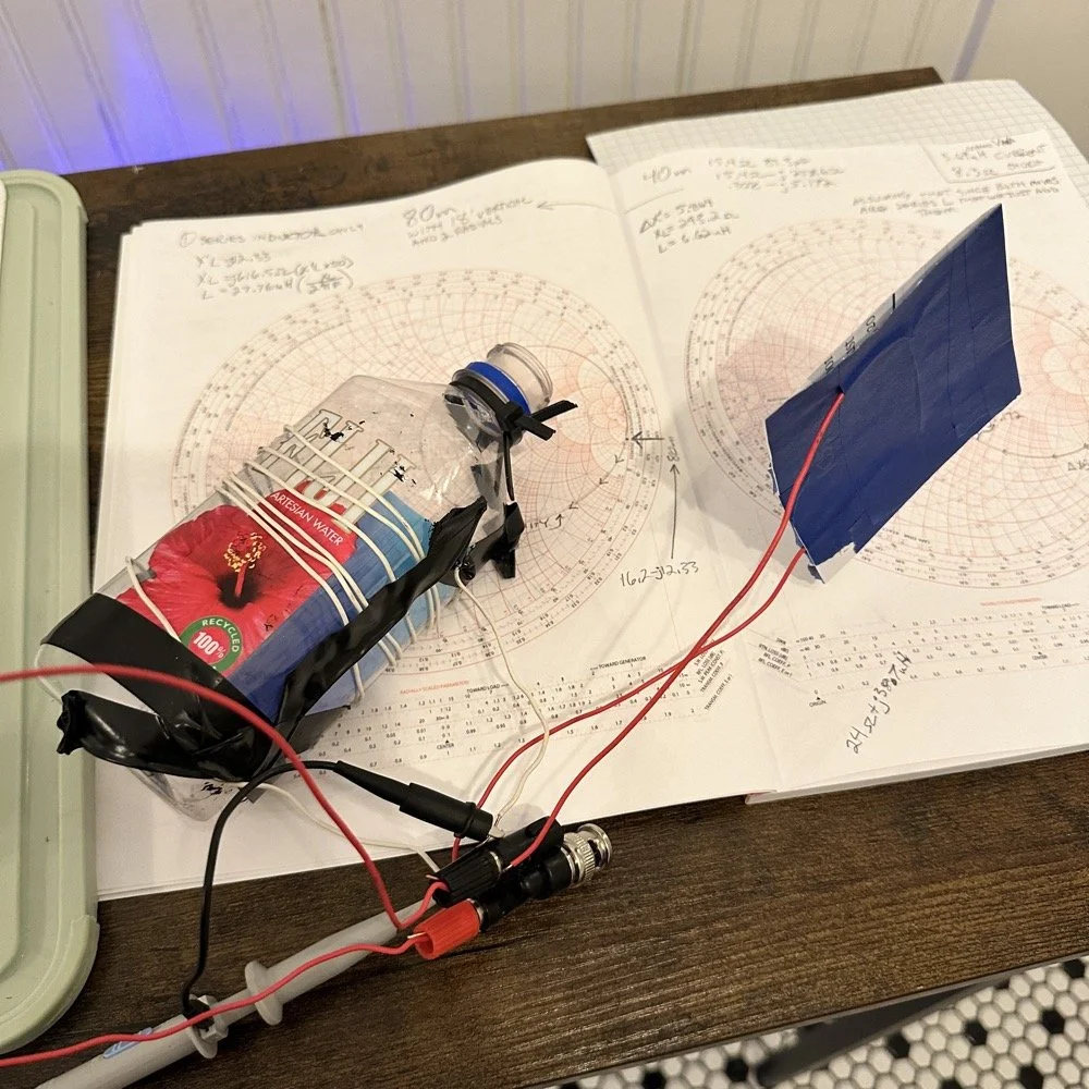
Once I had my brand spanking new capacitor made and trimmed to size (105pf), I setup a test fixture to do my test with. The test fixture is also expedient since it is all that I had was one of those “BNC to binding post” adapters and just used it as a sort of bread board to attach all the parts to the system. It worked, it was pretty janky, but it worked. All that we have here in reality is a parallel tank circuit. It will resonate at one frequency natively and I can measure that and then use a simple online calculator to see what the inductance is based on my capacitor value and the frequency of the tank circuit. How do I get it to resonate then? Simple, use a battery…
In the other video I had recently watched he showed simply setting the scope to trigger off of a voltage level close to the value of the battery which will allow the scope to capture the ringing of the tank circuit if you pulse it with a battery. I just took a AA out of my pocket flashlight and used it, set the trigger to normal and set the trigger level to about 1 volt and started touching the battery to the two red wires going out to the left in this photo below. This biased the tank circuit (simply applying a dc voltage across the capacitor and charging it) and I was rewarded with what you see below on the scope in the below photo. To be perfectly honest with you, I had done so much wrong in this process that I was honestly surprised that it worked. I even had to show it to Teresa and she had literally zero idea about what she was seeing here, but I had to show SOMEONE that it has actually worked!
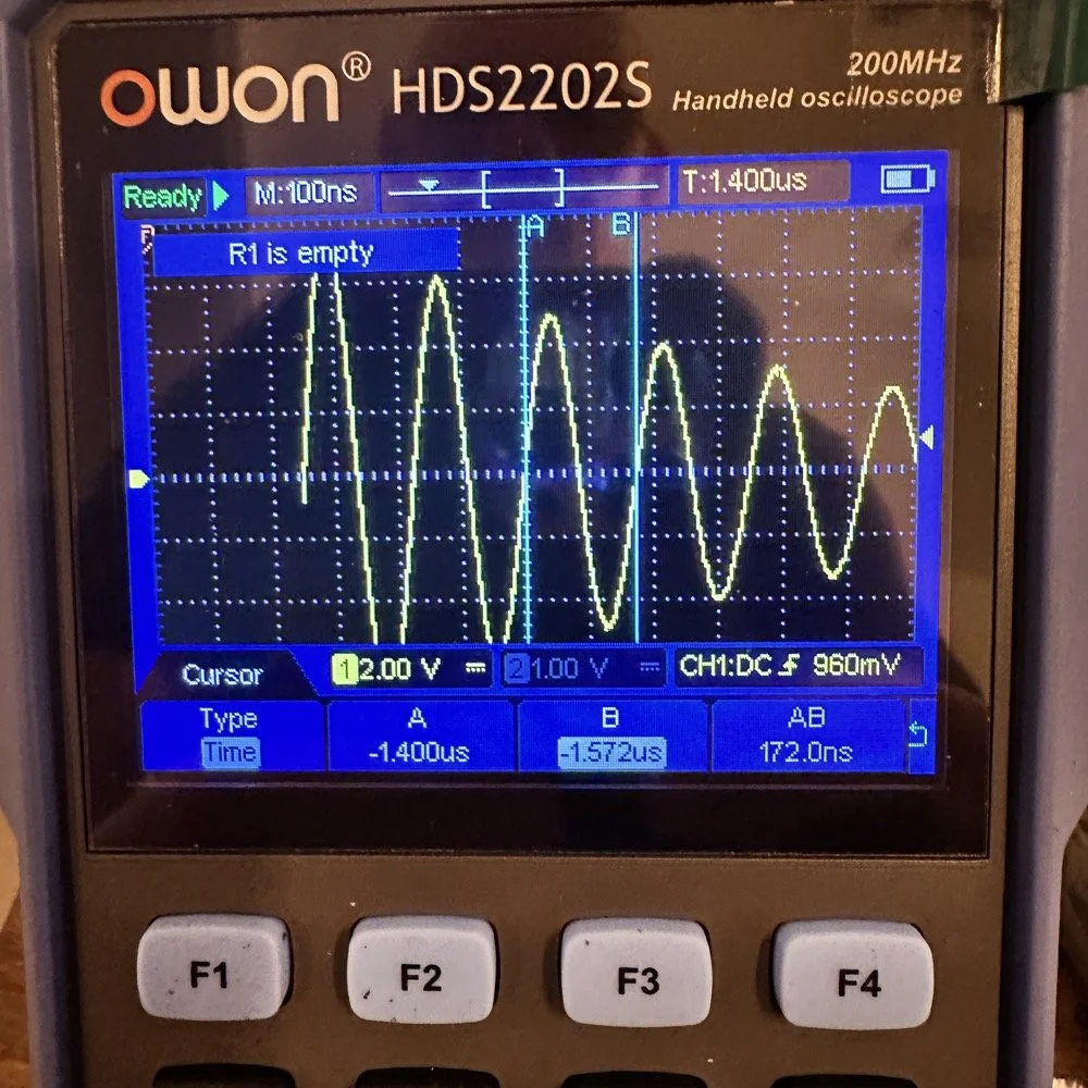
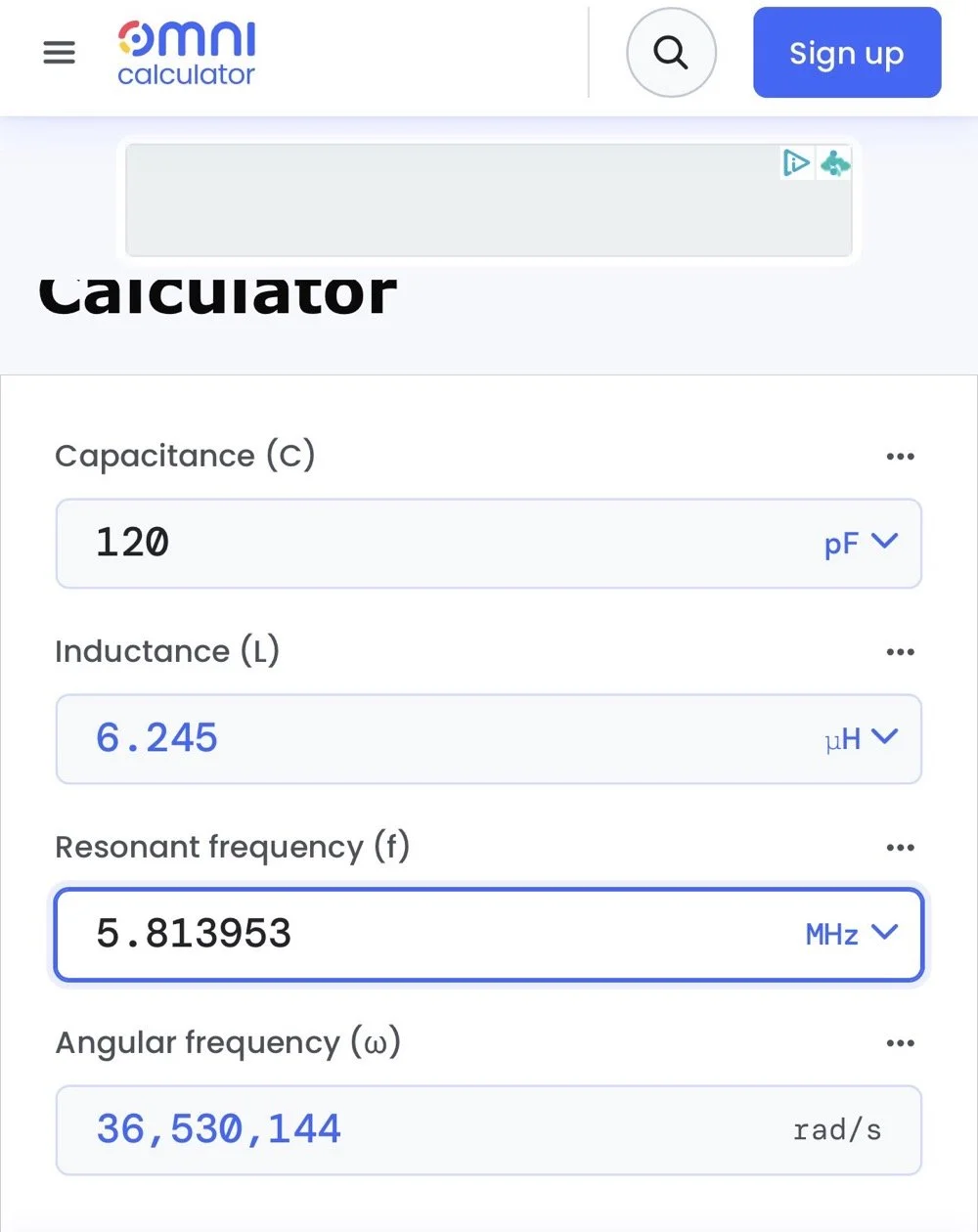
The ringing the scope captured is nice and clean and I was able to measure the period of the sine wave at 172 nanoseconds. Transforming the time into a frequency is easy, you simply invert the number or divide 1 by .000000172 and you get 5,813,953 hz. This frequency is not relevant to the ham bands but is only useful in telling us what the value of the inductor is, which is what we want anyway. As you can see from the screen shot below, this inductor is 6.245 uH (micro henrys). I did the plot on the smith chart for 40 meters for this antenna and came up with almost exactly this number, I came up with 6.62uH on the math. This also makes sense as I did this physical coil for the 213” (17.75’) WRC vertical and not this one that is longer that I am using now 221” (18.4’). Another possible reason for the variation from the measured and the plotted values is that my capacitor value could be slightly different from being moved around or being in proximity to metal or some such. You could touch the capacitor with your finger tip and the value would change so this is probably part of the variation…
I made this actual load coil by guessing to be honest, I did use the nanoVNA as a SWR meter when I made it and I would take off a coil or two and measure it and I simply walked the null in on the antenna for 40 meters that day. Now I know how to use a smith chart to do that math ahead of time. That is pretty cool.
Literally using trash to resonate as a tank circuit is kinda cool to be honest with you. The wires for the capacitor are simply taped to the aluminum foil, nothing more as I didn’t have a way to solder them together or anything like that. This was truly a temporary test fixture for experimentation.
The next logical step was to make an inductor for 60 meters and to hook it up to the antenna and measure it with the nanoVNA to see how close I could get it. This is where things started to go south…
First of all, I had problems replicating the same resistance and capacitance from that day at the POTA park. The photo of the VNA above shows what I am talking about. Now it is 1 ohm… yeah basically a dead short for the RF. But more importantly it is different from the day of my test which was about 10 ohms (if memory serves me) but basically this doesn’t matter when you get to the region of the smith chart that this plot is landing in. The capacitance is what really drives this position between these two numbers and it was virtually the same. The amount of inductance will be more for 1 ohm but not a whole lot more.
Well what happened when I hooked up the coil and the vertical and stuff in the driveway was a whole bunch of nothing! It just made a circle around the outside of the smith chart, which is bad if you don’t know. You want your line to go through the center of the chart at the frequency you want to use and if it goes around the outside it ain’t going through the middle!
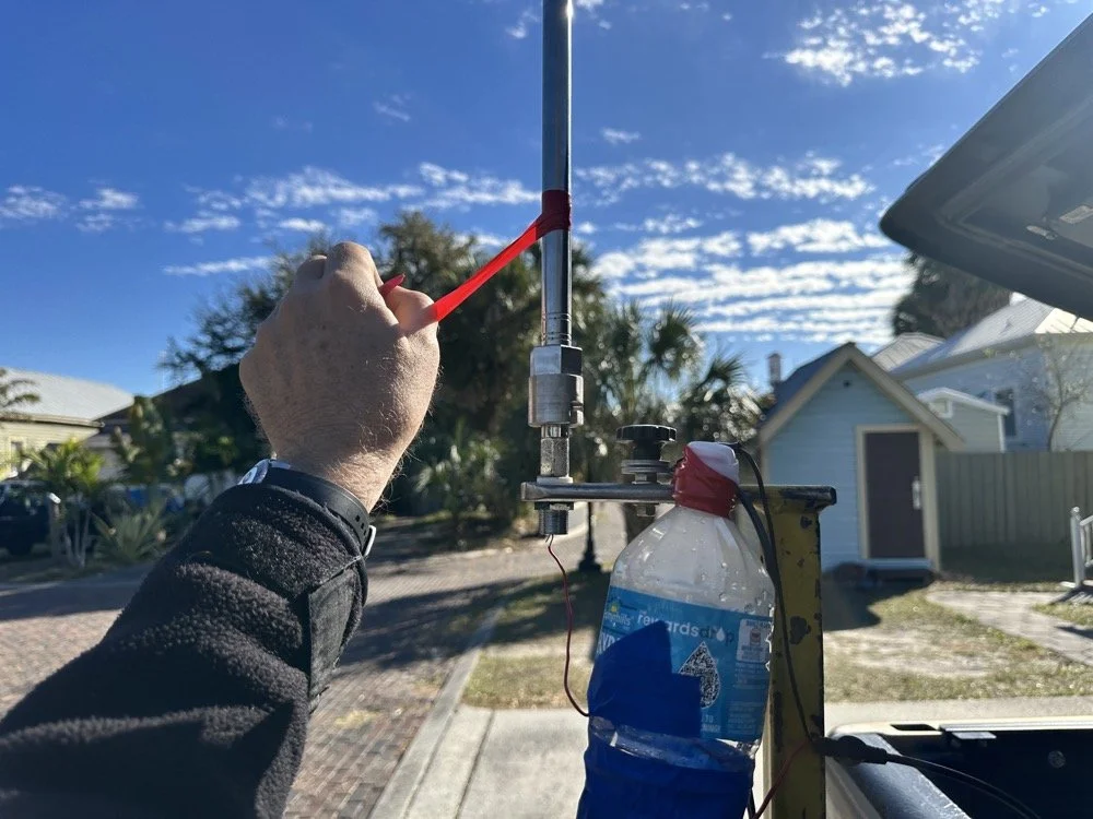
Deflated that I had probably done all that math wrong…again… I was about to throw in the towel when the wind blew and the plot on the nanoVNA moved towards the center! What just happened??? I start messing with this and that, as you can see in the photo above that the coil output wire is just poked into the coax port on the antenna. This has to be the worst way to make this connection, but if this is all you have, then this is what you do…
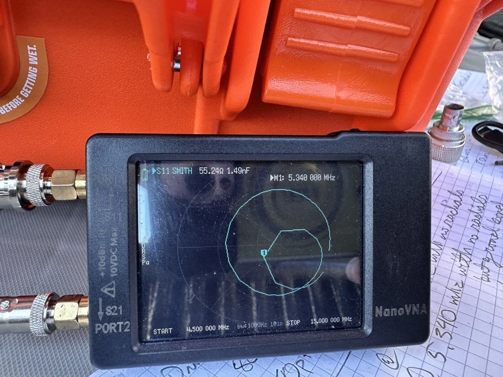
I could grab the vertical and that would make drastic changes to the smith plot, so I thought about moving the antenna without touching it and I found a roll of electrical tape and used that to tug on the vertical as it is in a QD mount (which is not a great connection to be honest that I have found). I even cleaned some stuff to no avail, but when I put the tape on the antenna and pulled it in certain directions, I would get the plot you see below. Notice the marker is at 5.340 mhz and at 55.2 ohms and just 1.49nf capacitive. This is less than 1.2 : 1 SWR and I am sure that it is off a little because of the system losses at this point. All the loose and dirty connections along with the random radial placement (I find this makes a pretty large difference with my systems) made getting repeatable results almost impossible. This told me that the coil worked though and that my math was not wrong! I had actually learned something here!
Once I figured this out and took a couple of photos for the blog, I tore the system back down and put it all away so I could get started on this write up about it. This has been an amazing process to do this and I learned way more than just how to do impedance matching with a smith chart. I learned that my system is way too inconsistent to simply make a coil and expect it to work in the system. If I had all the parts hard mounted in place with corrosion inhibiting paste on the connections then I could calculate this coil and it would drop right in. I was blown away by this and cant wait to find another use for my smith chart notebook. I hope this has helped you in some way either by simple entertainment or by learning something about smith charts and antennas, or maybe that there are YouTube videos about how to do this sort of stuff, either way, thank you for reading to here and I hope you come back for more of my ramblings in the future!
You can help support this website by using these Amazon Affiliate Links:
QRP/Portable Radios:
Antennas & Tuning:
CW Equipment:
Power & Accessories:
Organization & Transport:
BONUS ITEMS
73
WK4DS - David